4 How the machine computes
Lectures 1–3 showed how data is represented; now we open the box. The question of this chapter is mechanical: Given bits in memory, how does a computer actually compute? We build the answer from the bottom up - from a single switch to gates, from gates to an adder, from the adder to the Von Neumann machine, and finally through one complete instruction, register by register. This is among the densest lectures of the course, but it has a single thread you can hold on to throughout: A computer is many simple switches, arranged so that they fetch and carry out instructions stored in memory. Nothing more exotic than that.
4.1 From the switch to the gate
Chapter 2 introduced the transistor as the reason for binary; here it becomes a building material. A transistor is an electronic switch controlled by a voltage, with no moving parts: Gate LOW, no current flows - a 0; gate HIGH, current flows - a 1. Billions fit on one chip, each switching billions of times per second, and everything in this chapter is built from this one device.
Wire a few switches together and they can make decisions.
Definition 4.1 (Logic gates) A logic gate is a small transistor circuit computing a Boolean operation on one or two input bits: AND outputs 1 only if both inputs are 1; OR if either is; XOR if exactly one is; NOT inverts its single input; NAND is AND followed by NOT.

These are the same bitwise operations you met arithmetically in Chapter 2, now as hardware. The true/false algebra behind them is George Boole’s (1847); Claude Shannon’s insight of 1938 was that Boole’s algebra maps directly onto electrical switching circuits - the founding observation of digital electronics. One further fact is surprising enough to deserve its own paragraph: A single gate type suffices to build all the others. From NAND alone, \mathrm{NOT}\,a = \mathrm{NAND}(a,a); a\;\mathrm{AND}\;b = \mathrm{NOT}(\mathrm{NAND}(a,b)); and a\;\mathrm{OR}\;b = \mathrm{NAND}(\mathrm{NOT}\,a, \mathrm{NOT}\,b). (NOR is universal in the same way.) Because one gate type suffices, a chip can be manufactured from one repeated building block - an enormous practical advantage.
Build OR from NAND gates alone, and verify your construction on the input a = 1, b = 0.
Solution. Using the formula above: a\;\mathrm{OR}\;b = \mathrm{NAND}(\mathrm{NAND}(a,a), \mathrm{NAND}(b,b)) - three NAND gates, wired like this:
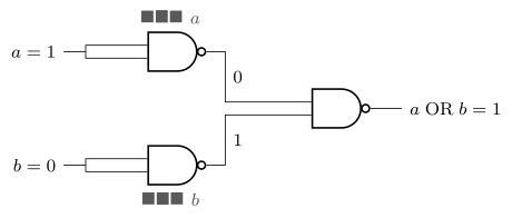
Trace the values: \mathrm{NAND}(1,1) = 0 (upper gate, acting as NOT a) and \mathrm{NAND}(0,0) = 1 (lower gate, NOT b); the final gate computes \mathrm{NAND}(0,1) = 1. Indeed 1\;\mathrm{OR}\;0 = 1.
Gates make decisions; can they also do arithmetic? Yes, and the construction is short enough to see whole.
Example 4.1 (The half-adder and the full adder) Add two bits a + b and look at Chapter 2’s addition table: The sum bit is 1 exactly when one of the inputs is 1 - that is XOR - and the carry bit is 1 exactly when both are - that is AND. So a half-adder is nothing but an XOR gate and an AND gate side by side. It cannot, however, accept a carry coming in from the column to its right. The full adder fixes that: It adds three bits a, b and a carry-in, with \text{sum} = a \oplus b \oplus c_{in} and carry-out = 1 whenever two or more inputs are 1; internally it is two half-adders plus an OR gate. Now chain eight full adders, carry-out to carry-in, and you have built the 8-bit adder that performs the byte addition of Chapter 2 - and, via two’s complement (Definition 2.2), its subtraction too. Binary arithmetic, in hardware, out of switches.
The same gates, repeated and combined, go further still: Comparison circuits test whether two values are equal or which is larger, and - the trick that will matter in Section 4.4 - feeding a gate’s output back to its own input lets it hold a bit: A flip-flop, the seed of memory. A whole CPU is millions of these gates arranged with care; nothing more exotic than switches.
4.2 The Von Neumann architecture, properly
Chapter 1 gave the blueprint in outline (Definition 1.4); now we can afford the full picture. The five hardware components are the control unit, the arithmetic logic unit (ALU), memory, input and output - where control unit, ALU and a handful of registers together form the CPU. (The operating system, note, is software, not one of the five.) Inside the CPU the division of labour is clean: The control unit reads each instruction and issues the signals that carry it out; the ALU performs the arithmetic and logic of the previous section - it is, quite literally, built of the gates and adders above; the registers are a few tiny, very fast stores for the values in use right now.
The defining idea deserves restating with the weight it carried in 1945. Earlier machines were rewired by hand for each new task. Von Neumann’s insight - the stored-program principle - was to store the program in the same memory as the data: The same hardware can then run any program, just by loading different bits. A program is data that the CPU chooses to interpret as instructions. Contemporaries summarised it in three words: Software was born.
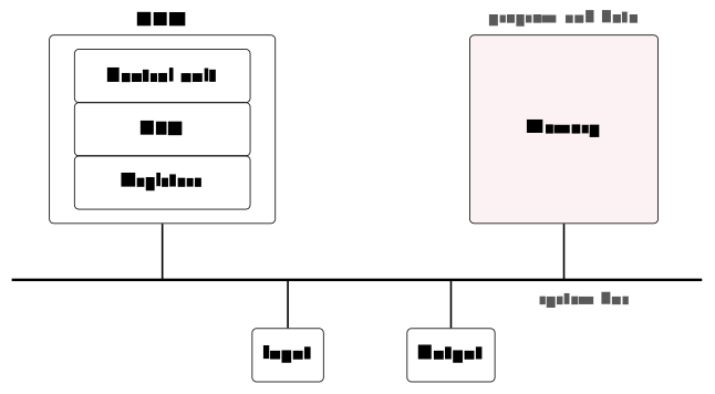
The design has a cost, and it has a name. Because every instruction and every piece of data crosses the same single bus between CPU and memory, the bus limits throughput: The CPU often waits on memory. This is the Von Neumann bottleneck, and the caches of Section 4.4 exist largely to relieve it. The classical alternative, the Harvard architecture, splits the paths - separate memories and buses for instructions and data, accessible simultaneously and therefore faster - and survives in microcontrollers and signal processors. Modern CPUs are a pragmatic hybrid: Von Neumann as the programmer sees them, but with split instruction and data caches inside.
Two amendments complete the modern picture. First, the GPU: A second processor specialised for doing the same operation on lots of data at once. Where the CPU has a few powerful cores tuned for varied, sequential work, the GPU has thousands of small ones all performing the same step - ideal for graphics and, today, for AI and other massively parallel mathematics; it trades flexibility for sheer parallel throughput. Second, multi-core: When clock speeds stopped rising (Section 4.5 says why), makers began packing several full cores onto one CPU, running different programs - or parts of one - truly simultaneously. The catch is honest: Software must be written to use the cores; not everything parallelises.
4.3 The HIDAS cycle: One instruction, step by step
Before watching the CPU run, one translation question. The CPU runs only binary; how does c = a + b; become bits? In two steps: A compiler translates the high-level statement into assembly - human-readable mnemonics such as ADD R3, R1, R2 - and an assembler turns each mnemonic into machine code: A binary opcode naming the operation plus a few bits naming the registers. The bits are the very same bits we met in Chapter 2 - only now they are the program (the stored-program principle, seen from below).
The cycle itself depends on a few special registers: The program counter (PC) holds the memory address of the next instruction to fetch; the instruction register (IR) holds the instruction currently being carried out; the accumulator (A) holds the current working value. Registers are the fastest memory in the machine - faster even than cache - because they sit inside the CPU itself.
Definition 4.2 (The HIDAS cycle) The CPU executes every instruction through five steps, repeated endlessly: Holen (fetch the instruction at the address in PC into IR) - Inkrementieren (increment PC to point at the next instruction) - Dekodieren (decode: Work out what the instruction in IR means) - Ausführen (execute the operation) - Speichern (store the result). The mnemonic keeps its German step names; Example 1.3 in Chapter 1 was this same cycle in its compressed three-step form, fetch–decode–execute, with the increment and store steps folded in.
Example 4.2 (Tracing LOAD 256) Set the stage: Memory address 100 contains the instruction LOAD 256 (“copy the value stored at address 256 into the accumulator”), address 256 contains the value 47, and the registers start at \mathrm{PC}=100, IR and A empty. Now run one full cycle. H: The control unit puts \mathrm{PC}=100 on the address bus and reads memory; LOAD 256 comes back and lands in IR. I: PC is increased to 101 - now, not later. Why before executing? Because if this instruction turns out to be a jump, the execute step will overwrite PC with the jump target; incrementing afterwards would undo the jump. D: The control unit examines IR, recognises the operation LOAD and the operand 256, and prepares the control signals - no register changes. A: Memory at address 256 is read, yielding 47. S: 47 is placed into A. End state: \mathrm{PC}=101, \mathrm{A}=47, and the CPU returns to H.
Memory address 200 holds the instruction LOAD 300; address 300 holds the value 13; the registers start at \mathrm{PC}=200, IR and A empty. Walk through H–I–D–A–S and give the end state of PC, IR and A.
Solution. H: The instruction at address 200 - LOAD 300 - is fetched into IR. I: PC becomes 201. D: The control unit recognises LOAD with operand 300. A: Memory at 300 is read, yielding 13. S: 13 lands in A. End state: \mathrm{PC}=201, \mathrm{IR}=\texttt{LOAD 300}, \mathrm{A}=13.
What paces this loop is the clock: A steady pulse driving the CPU from step to step. A 3 GHz CPU ticks three billion times per second; each HIDAS step is paced by those ticks, and multiple cores run several such cycles in parallel. Hold on to the perspective this gives: The whole machine, however sophisticated, is this same tiny cycle repeated at enormous speed.
Tanenbaum’s favourite description of the HIDAS loop is worth carrying around: The CPU is an interpreter - a tireless clerk running an endless loop of “fetch the next order, work out what it says, do it, repeat”. Nothing about the clerk changes when the program changes; only the orders do. That framing explains two things at once. First, why the stored-program principle is so powerful: Swap the orders in memory and the same clerk performs a completely different job. Second, why the tower-of-levels picture from Chapter 1 works at all: Any level can be realised by an interpreter running on the level below - exactly what a Python interpreter, a Java virtual machine or an emulator for an old game console does in software, and what the CPU itself does in hardware. Interpretation all the way down.
(Tanenbaum & Austin, 2013, ch. 1–2)
4.4 Memory and addressing
Instructions need data, and the data lives in memory - which is best pictured as one very long row of numbered cells, each holding one byte and each carrying a unique address. The CPU selects a cell by placing its address on the address bus. How much memory can it reach? With an N-bit address bus, 2^N distinct locations: A 32-bit bus reaches 2^{32} \approx 4 billion bytes - 4 GB - which is precisely why 32-bit systems topped out there, and one more reason the world moved to 64-bit words (Definition 1.2).
One genuinely counter-intuitive subtlety hides in multi-byte values: In which order are their bytes stored?
Example 4.3 (Endianness) Store the 32-bit value 0x12345678 at addresses 100–103. A little-endian machine puts the least-significant byte at the lowest address: 100 holds 78, then 56, 34, 12. A big-endian layout stores them in reading order: 12 34 56 78. Both denote the same value - endianness is a convention, not a difference in meaning - but the conventions collide exactly where data changes hands: X86 and ARM processors are little-endian, while network protocols transmit big-endian (“network byte order”), a fact that returns in the networking modules.
The working memory itself, RAM, is defined as much by what it is not. It is volatile (contents lost at power-off), random-access (any cell reachable in the same time) and much faster than SSD or HDD; it is not permanent storage, and not as fast as the CPU’s registers or cache. Volatile is the word to underline: It is why unsaved work disappears when the power fails - the work lived only in RAM.
RAM is one rung on the ladder you met in Chapter 1, the memory hierarchy: Registers, cache, RAM, SSD/HDD - each level faster, smaller and costlier than the one below. Now we can explain the rung between registers and RAM properly. The cache is a small, fast copy of the data the CPU is most likely to need next: A cache hit means the data is already there (very fast); a miss means waiting for RAM. The startling fact is that hits run at 90–99 % - because of locality: Programs tend to reuse the same data (temporal locality) and nearby data (spatial locality), so a small cache covers most accesses. The cache is how modern CPUs hide much of the Von Neumann bottleneck. It comes in levels: L1, tiny and fastest, inside each core (often split for instructions and data - the Harvard hybrid from above); L2, larger, still per core; L3, largest, shared by all cores. The CPU checks L1, then L2, then L3, then RAM, stopping at the first level that holds the data.
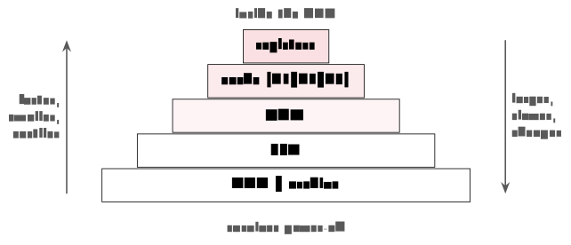
At the bottom sits mass storage, large and non-volatile. The hard disk (HDD) - spinning magnetic platters and a moving read head - is cheap per gigabyte but slow and mechanical; the solid-state drive (SSD) - flash memory, no moving parts - is much faster and more robust at a higher price per gigabyte, and has largely replaced HDDs in laptops. And one last hardware fact with a security-flavoured moral: Stored bits can flip - cosmic rays and electrical noise occasionally do it - so ECC memory adds check bits to every word and can detect, and usually correct, a single flipped bit automatically. It is standard in servers, where silent data corruption is unacceptable; the underlying idea returns as the parity and CRC checks of the networking modules.
4.5 Performance and trends
Step back, finally, to the trend behind all this growth - picking up the timeline of Chapter 1 with the vocabulary to appreciate it. Moore’s Law, Gordon Moore’s 1965 observation, held that transistor counts double roughly every two years, and for decades it did: From the Intel 4004’s 2 300 transistors (1971) through the Pentium 4’s 42 million and the Core i7’s 1.2 billion to Apple’s M-series at 16 and now 28 billion. On a logarithmic scale the points fall on a straight line - exponential growth - and any dashed continuation to 2030 (~50 billion) is an assumption, not a measurement.
The second half of the story matters just as much. For decades, each generation brought higher clock speeds essentially for free; around 2005, rising heat capped the clocks, and designers added cores instead - the multi-core turn of Section 4.2. Today transistors approach atomic scales, and the gains come from parallelism, from caches, and from specialised silicon - GPUs, AI accelerators, chiplet designs - rather than raw clock. The free lunch of ever-faster single cores is over; performance now depends on using many cores well, which is a software problem, and a fitting note on which to hand over to next week’s subject.
Three two-minute checks from the lecture, worth redoing cold: 1011\,0010\;\mathrm{XOR}\;1100\,1110 (answer: 0111\,1100 - and notice it is Example 4.1’s sum bits, byte-wide). A cycle starts at \mathrm{PC}=100 with LOAD 256, and address 256 holds 9 - after one HIDAS cycle, \mathrm{PC}=101 and \mathrm{A}=9. A 16-bit address bus reaches 2^{16} = 65\,536 locations.
Before Lecture 5 (Operating systems). Read the Module 5 chapter in the textbook (Readings.xlsx for the pages). Try this: Open Task Manager or Activity Monitor and watch how memory and CPU are shared among the programs you have running. And think about the question that opens next week: If the CPU can run only one HIDAS cycle at a time, how can a computer appear to run many programs at once?
4.6 Summary
Everything is switches: Transistors form gates (Definition 4.1); NAND alone can build every logic function; XOR and AND side by side make a half-adder, full adders chain into the byte arithmetic of Chapter 2 (Example 4.1), and a fed-back gate can even remember a bit. The Von Neumann architecture arranges the result - control unit, ALU and registers as the CPU, plus memory, input and output - around the stored-program principle: Programs live in memory as data, so loading different bits gives the same machine a different job, at the price of the shared-bus bottleneck that caches exist to hide. Every instruction runs through the HIDAS cycle (Definition 4.2, Example 4.2) - fetch, increment, decode, execute, store - paced by a clock at billions of ticks per second. Memory is addressed bytes: An N-bit bus reaches 2^N cells, endianness fixes the byte order (Example 4.3), RAM is fast and volatile, and the hierarchy - registers, L1/L2/L3 cache, RAM, SSD/HDD - turns locality into 90–99 % cache hit rates. And Moore’s Law explains both the eighty-year boom and the present turn: Clocks capped by heat, gains now from cores and specialised chips. Next week: The software that makes one machine appear to be many - the operating system.
Interactive checks
A round of quick interactive drills - instant feedback, all in your browser, nothing recorded. Every task has a show-solution button; clicking it straight away is no fun.
Self-check
Exercise 4.1 (Building gates from NAND) Using only NAND gates, construct NOT and AND, writing each as a formula.
Exercise 4.2 (Half-adder versus full adder) What exactly can a full adder do that a half-adder cannot - and why does that one capability make multi-bit addition possible?
Exercise 4.3 (Why increment before execute) In the HIDAS cycle, why is the program counter incremented before the execute step rather than after it?
Exercise 4.4 (Endianness in memory) The 32-bit value 0xA1B2C3D4 is stored little-endian at addresses 200–203. Which byte sits at address 200, and which at 203?
Exercise 4.5 (Locality and the cache) Explain, using the two kinds of locality, why a cache far smaller than RAM can nevertheless serve 90–99 % of memory accesses.
- \mathrm{NOT}\,a = \mathrm{NAND}(a,a); for AND, feed \mathrm{NAND}(a,b) into that NAND-built NOT: a\,\mathrm{AND}\,b = \mathrm{NOT}(\mathrm{NAND}(a,b)). (2) Accept a carry-in; only with it can adders chain carry-to-carry into an 8-, 16- or 64-bit adder - the half-adder has no third input for the neighbouring column’s carry. (3) Because a jump instruction overwrites PC with its target during execute; incrementing afterwards would destroy the jump. Incrementing first makes “next instruction” the default that execute may then override. (4) Little-endian stores the least-significant byte lowest: Address 200 holds
D4, address 203 holdsA1. (5) Temporal locality: Recently used data is likely to be used again, so keeping it cached pays off; spatial locality: Nearby addresses are likely next, so caches load whole neighbouring blocks. Together they concentrate most accesses on a small working set that fits in the cache.
We now own the whole machine: Gates, adders, registers, and a CPU that executes exactly one instruction at a time - and precisely there hangs the question this chapter left open on purpose. How can such a machine run a browser, a music player and a dozen background tasks at once? Chapter 5 answers it with the operating system, built directly on the hardware met here: The registers saved in every context switch, and the interrupt that hands the machine back to its manager.